Good afternoon
This article is devoted to solving the question of how to compare two tables in Excel, or at least two columns. Yes, working with tables is convenient and good, but when you need to compare them, it is quite difficult to do this visually. Perhaps you can visually sort a table of up to a dozen or two, but when they exceed thousands, then you will need additional analysis tools.
Alas, there is no magic wand with which everything will be done in one click and the information will be checked; it is necessary to prepare data, and write formulas and other procedures that allow you to compare your tables.
Let's look at several options and possibilities for comparing tables in Excel:
The easy way
This is the simplest and most basic way to compare two tables. It is possible to compare both numeric and text values in this way. For example, let’s compare two ranges of numerical values, just by writing in the next cell the formula for their equality =C2=E2, as a result, if the cells are equal, we get the answer "TRUE", and if there are no matches, there will be "LIE". Now, by simple auto-copying, we copy it onto our formula that allows us to compare two columns in Excel and see the difference.

Quickly highlight values that are different
This is also not a very cumbersome method. If you just need to find and verify the presence or absence of differences between tables, you need to go to the “Home” tab, select the “Find and Select” menu button, having previously selected the range where you want to compare two tables in Excel. In the menu that opens, select “Select a group of cells...” and in the dialog box that appears, select "differences by line".

Compare two tables in Excel using conditional formatting
A very good way in which you can see in highlighted colors the values that differ when comparing two tables. You can apply on the tab "Home" by pressing the button "Conditional Formatting" and select from the list provided "Rule Management". In the dialog box "Conditional Formatting Rules Manager", press the button "Create Rule" and in a new dialog box "Create a formatting rule", select a rule. In field "Change rule description" enter the formula =$C2<>$E2 to determine the cell that needs to be formatted and press the button "Format".
 We determine the style of how our value that meets the criterion will be formatted.
  Now our newly created rule has appeared in the list of rules, you select it, click "OK".
And the entire rule was applied to our range, where we are trying to check the similarity of two tables, and the differences became visible, to which conditional formatting was applied.

How to compare two tables in Excel using the COUNTIF function and rules
All of the above methods are good for ordered tables, but when the data is not ordered, other methods are needed, one of which we will now consider. Let's imagine, for example, we have 2 tables whose values are slightly different and we need to compare these tables to determine the value that is different. Select the value in the range of the first table and on the tab "Home", menu item "Conditional Formatting" and click on the item in the list "Create a rule...", select a rule "Use a formula to determine which cells to format", enter the formula = ($C$1:$C$7;C1)=0 and select the conditional formatting format. 
The formula checks the value from a specific cell C1 and compares it to the specified range $C$1:$C$7 from the second column. We copy the rule to the entire range in which we compare tables and get values highlighted in cells that do not repeat.
How to compare two tables in Excel using the VLOOKUP function
In this option we will use , which will allow us compare two tables for coincidences. To compare two bars, enter the formula =VLOOKUP(C2,$D$2:$D$7,1,0) and copy it to the entire range being compared. This formula sequentially begins to check whether there are repetitions of the value from column A in column B, and accordingly returns the value of the element, if it was found there, if the value is not found, we get .

How to compare two tables in Excel IF functions
This option involves the use of a logical one, and the difference between this method is that to compare two columns, not the entire column will be used, but only that part of it that is needed for comparison.
For example, let’s compare two columns A and B on the worksheet; in the adjacent column C we enter the formula: =IF( (MATCH(C2,$E$2:$E$7,0));"";C2) and copy it to the entire . This formula allows you to view sequentially whether certain elements from the specified column A are in column B and returns the value if it was found in column B.

Compare two tables using VBA macro
There are many ways to check two tables for similarity , but some options are only possible using VBA macros. Macros for comparing two tables , unifies this process and significantly reduces the time spent on data preparation. Based on the problem you are solving and your knowledge of VBA macros, you can create any variant of macros. Below I have given the method indicated on the official Microsoft page. You need to create a VBA code module and enter the code:
Sub Find_Matches() Dim CompareRange As Variant, x As Variant, y As Variant " Set the CompareRange variable equal to the range being compared Set CompareRange = Range("B1:B11") " If the range being compared is on a different sheet or workbook, " use the following syntax " Set CompareRange = Workbooks("Book2"). _ " Worksheets("Sheet2").Range("B1:B11") " " Compare each element in the selected range with each element of the " variable CompareRange For Each x In Selection For Each y In CompareRange If x = y Then x.Offset( 0, 2) = x Next y Next x End Sub
Sub Find_Matches() Dim CompareRange As Variant , x As Variant , y As Variant " Setting the CompareRange variable to the range being compared Set CompareRange = Range("B1:B11") " If the range being compared is on a different sheet or workbook, " use the following syntax " Set CompareRange = Workbooks ("Book2") . _ Hotkey shortcut Alt+F8. In the new dialog box, select your macro Find_similar and do it. Comparisonusing the Inquire add-on
This compare option became available with the release of the 2013 version of Excel, the editor was added Inquire add-on, which will allow you to analyze and compare two Excel files. This method is good when you need to compare two files, in case your colleague was working on a book and made some changes. To determine these changes you need a tool WorkbookCompare in the add-inInquire. Well, we’ve looked at 8 ways to compare two tables in Excel; these options will help you solve your analytical problems and simplify your work. I was glad to help you!
|
Sometimes there is a need to compare two MS Excel files. This may be finding discrepancies in prices for certain items or changing any indications, it doesn’t matter, the main thing is that it is necessary to find certain discrepancies.
It would not be amiss to mention that if there are a couple of records in the MS Excel file, then there is no point in resorting to automation. If the file contains several hundred, or even thousands of records, then it is impossible to do without the help of the computing power of a computer.
Let's simulate a situation where two files have the same number of lines, and the discrepancy must be looked for in a specific column or in several columns. This situation is possible, for example, if you need to compare the price of goods according to two price lists, or compare measurements of athletes before and after the training season, although for such automation there must be a lot of them.
As a working example, let's take a file with the performance of fictitious participants: 100-meter run, 3000-meter run, and pull-ups. The first file is a measurement at the beginning of the season, and the second is the end of the season.
The first way to solve the problem. The solution is only using MS Excel formulas.
Since the records are arranged vertically (the most logical arrangement), it is necessary to use the function. If you use horizontal placement of records, you will have to use the function.
To compare 100 meter running performance, the formula is as follows:
=IF(VLOOKUP($B2,Sheet2!$B$2:$F$13,3,TRUE)<>D2;D2-VLOOKUP($B2;Sheet2!$B$2:$F$13,3,TRUE);"No difference")
If there is no difference, a message is displayed that there is no difference; if there is a difference, then the value at the end of the season is subtracted from the value at the end of the season.
The formula for the 3000 meter run is as follows:
=IF(VLOOKUP($B2,Sheet2!$B$2:$F$13,4,TRUE)<>E2;"There is a difference";"There is no difference")
If the final and initial values are not equal, a corresponding message is displayed. The formula for pull-ups can be similar to any of the previous ones; there is no point in giving it additionally. The final file with the discrepancies found is shown below.
A little clarification. To make the formulas easier to read, the data from the two files was moved into one (on different sheets), but this could not have been done.
Video comparing two MS Excel files using and functions.
The second way to solve the problem. Solution using MS Access.
This problem can be solved if you first import MS Excel files into Access. As for the method of importing external data itself, there is no difference in finding different fields (any of the presented options will do).
The latter is a connection between Excel and Access files, so when you change data in Excel files, discrepancies will be found automatically when you run a query in MS Access.
The next step after importing is to create relationships between tables. As a connecting field, select the unique field “Item No.”
The third step is to create a simple select query using the Query Builder.
In the first column we indicate which records need to be displayed, and in the second - under what conditions the records will be displayed. Naturally, for the second and third fields the actions will be similar.
Video comparing MS files to Excel using MS Access.
As a result of the manipulations performed, all records are displayed, with different data in the field: “Running 100 meters.” The MS Access file is presented below (unfortunately, SkyDrive does not allow embedding as an Excel file)
These two methods exist for finding discrepancies in MS Excel tables. Each has both advantages and disadvantages. Obviously, this is not an exhaustive list of comparisons between the two Excel files. We are waiting for your suggestions in the comments.
The Inquire add-in for Excel 2013 allows you to compare and analyze Excel documents to look for relationships, erroneous formulas, and differences between .xlsx files. Let's look at the moments when this add-in may be useful to you and how to use it.
Launching the Inquire add-in
The Inquire add-in for Excel comes standard with Excel 2013 and does not require additional installation packages. It is enough to enable it in add-ons. Earlier versions of Excel do not support this add-in. In addition, at the time of writing, the add-on was only available in English.
To launch Inquire, go to the tab File –> Options. In the dialog box that appears, select the tab Add-ons, in the dropdown menu Control select Add-onsCOM and click the button Go. A window will appear Add-ons for the component object model (COM), where you will need to check the box Inquire and press the button OK.

After launching the add-in, a new tab will appear on the ribbon Inquire.

Let's see what benefits this add-on gives us.
Workbook Analysis
Workbook analysis is used to identify workbook structure, formulas, errors, hidden sheets, etc. To use this tool, go to the group Report and click the button Workbook Analysis. The result of the add-in is presented below.

Surely many people paid attention to the point Veryhiddensheets(Very hidden sheets). This is not a joke, in Excel you can actually hide a sheet “well” using the VisualBasic editor. We will talk more about this in our subsequent articles.
Linking to Worksheets
In Group Diagram, There are three tools for defining connections between workbooks, sheets and cells. They allow you to indicate relationships between Excel elements. This functionality can be useful when you have a large number of cells with links to other books. Trying to unravel this tangle can take a significant amount of time, while the Inquire add-in allows you to visualize data dependencies.
To build a dependency diagram, in the group Diagram select one of the items WorkbookRelationship, WorksheetRelationship or CellRelationship. The choice will depend on what kind of dependency you want to see: between workbooks, sheets or cells.
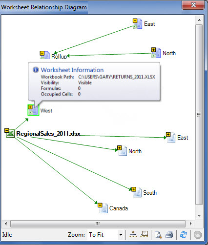
In the picture below you will see the workbook relationship diagram that Excel produced when I clicked the button WorkbookRelationship.

Comparing two files
The next Inquire add-in tool for Excel is Compare– allows you to compare two files cell by cell and point out any differences between them. This tool may be needed when you have several revisions of the same file and need to understand what changes were made to the latest versions.
To use this tool you will need two files. In Group Compare choose CompareFiles. In the dialog box that appears, we must select the files that we want to compare and click the button Compare.

In our case, these are two identical files, to one of which I deliberately made some changes.
After some deliberation, Excel will produce the result of the comparison, where the differences between the two tables will be indicated in color. In this case, the cell color will be different depending on the type of cell difference (differences can be generated due to values, formulas, calculations, etc.).

Cleaning up unnecessary formatting
This tool allows you to clean up unnecessary formatting from cells in a workbook, such as cells that are formatted but do not contain values. Tool Clean Excess Cell Formatting will help “amateurs” to fill the entire row of a workbook with color, instead of filling specific rows of the table.

To use the tool, go to the tab Inquire to the group Miscellaneous and select Clean Excess Cell Formatting. In the window that appears, you need to select the area for clearing excess formatting - the entire workbook or the active sheet - click OK.

Cleaning up unnecessary formatting will reduce file size and increase productivity.
Workbook passwords
If you intend to analyze password-protected workbooks, you will need to specify them in Workbook Passwords.
Bottom line
The Inquire add-in for Excel contains several interesting tools that will help you improve the accuracy and integrity of your workbooks. If you use Excel 2013, it makes sense to pay attention to this add-in.
Say you want to compare versions of a workbook, analyze a workbook for problems or inconsistencies, or see links between workbooks or worksheets. If Microsoft Office 365 or Office Professional Plus 2013 is installed on your computer, the Spreadsheet Inquire add-in is available in Excel.
You can use the commands in the Inquire tab to do all these tasks, and more. The Inquire tab on the Excel ribbon has buttons for the commands described below.
If you don't see the Inquire tab in the Excel ribbon, see Turn on the Spreadsheet Inquire add-in .
Compare two workbooks
The Compare Files command lets you see the differences, cell by cell, between two workbooks. You need to have two workbooks open in Excel to run this command.
Results are color coded by the kind of content, such as entered values, formulas, named ranges, and formats. There"s even a window that can show VBA code changes line by line. Differences between cells are shown in an easy to read grid layout, like this:

The Compare Files command uses Microsoft Spreadsheet Compare to compare the two files. In Windows 8, you can start Spreadsheet Compare outside of Excel by clicking Spreadsheet Compare on the Apps screen. In Windows 7, click the Windows Start button and then > All Programs > Microsoft Office 2013 > Office 2013 Tools > Spreadsheet Compare 2013.
To learn more about Spreadsheet Compare and comparing files, read Compare two versions of a workbook.
Analyze a workbook
The Workbook Analysis command creates an interactive report showing detailed information about the workbook and its structure, formulas, cells, ranges, and warnings. The picture here shows a very simple workbook containing two formulas and data connections to an Access database and a text file.

Show workbook links
Workbooks connected to other workbooks through cell references can get confusing. Use the to create an interactive, graphical map of workbook dependencies created by connections (links) between files. The types of links in the diagram can include other workbooks, Access databases, text files, HTML pages, SQL Server databases, and other data sources. In the relationship diagram, you can select elements and find more information about them, and drag connection lines to change the shape of the diagram.
This diagram shows the current workbook on the left and the connections between it and other workbooks and data sources. It also shows additional levels of workbook connections, giving you a picture of the data origins for the workbook.

Show worksheet links
Got lots of worksheets that depend on each other? Use the to create an interactive, graphical map of connections (links) between worksheets both in the same workbook and in other workbooks. This helps give you a clearer picture of how your data might depend on cells in other places.
This diagram shows the relationships between worksheets in four different workbooks, with dependencies between worksheets in the same workbook as well as links between worksheets in different workbooks. When you position your pointer over a node in the diagram, such as the worksheet named "West" in the diagram, a balloon containing information appears.
Show cell relationships
To get a detailed, interactive diagram of all links from a selected cell to cells in other worksheets or even other workbooks, use the Cell Relationship tool. These relationships with other cells can exist in formulas, or references to named ranges. The diagram can cross worksheets and workbooks.
This diagram shows two levels of cell relationships for cell A10 on Sheet5 in Book1.xlsx. This cell is dependent on cell C6 on Sheet 1 in another workbook, Book2.xlsx. This cell is a precedent for several cells on other worksheets in the same file.

To learn more about viewing cell relationships, read See links between cells.
Clean excess cell formatting
Ever open a workbook and find it loads slowly, or has become huge? It might have formatting applied to rows or columns you aren't aware of. Use the Clean Excess Cell Formatting command to remove excess formatting and greatly reduce file size. This helps you avoid "spreadsheet bloat," which improves Excel"s speed.
Manage passwords
If you"re using the Inquire features to analyze or compare workbooks that are password protected, you"ll need to add the workbook password to your password list so that Inquire can open the saved copy of your workbook. Use the Workbook Passwords command on the Inquire tab to add passwords, which will be saved on your computer. These passwords are encrypted and only accessible by you.
Compare Spreadsheets for Excel is a powerful and convenient tool for comparing Microsoft Excel files.
Why is this needed and how does it work:
For example, you receive monthly price lists of the following type from your partners:
September
October
A quick look at them seems that the price lists have not changed. Of course, you can spend a longer time on a detailed comparison of all product items and prices in order to understand whether there are any changes or not. However, let's try to delegate this task Compare Spreadsheets for Excel::
- Run the program (it is not necessary to open the tables being compared in Microsoft Excel).
- Specify tables or ranges of cells to compare;
- Select alignment options for comparison (by rows, columns or without alignment);
- Specify what you want to compare: cell values or formulas;
- Set options for highlighting different cells (background color and/or cell border color and style).
Five simple steps, a few seconds of time and you have the following report:

The program found all the changes in the latest price list: a new product (highlighted in light green) and changed prices (cells with a red border).
Now imagine that your files do not have 20 rows and 8 columns. Correctly comparing two large documents manually is a very difficult task. But all the difficulties disappear if you compare Microsoft Excel spreadsheets using Compare Spreadsheets for Excel!
Program features
- Work with files, tables, or a selected range of cells.
- Working with files without opening them in Microsoft Excel.
- A simple and convenient interface of the program in the form of a wizard.
- Display comparison results in the form of a customizable, convenient and visual report.
- Ability to compare arbitrary cells in the resulting report.
- Comparison by cell values or formulas.
Download demo version
You can download a demo version of Compare Spreadsheets for Excel (17906 KB) to test it before purchasing:
Program registration
The demo version of Compare Spreadsheets for Excel has no limitations. If you want after the end of the 20-day demo period, then you need to register the program. You can register Compare Spreadsheets for Excel online by choosing a payment method that is convenient for you.