Types of dispersions:
Total variance characterizes the variation of a characteristic of the entire population under the influence of all those factors that caused this variation. This value is determined by the formula
where is the overall arithmetic mean of the entire population under study.
Average within-group variance indicates a random variation that may arise under the influence of any unaccounted factors and which does not depend on the factor-attribute that forms the basis of the grouping. This variance is calculated as follows: first, the variances for individual groups are calculated (), then the average within-group variance is calculated:
 where n i is the number of units in the group
Intergroup variance(variance of group means) characterizes systematic variation, i.e. differences in the value of the studied characteristic that arise under the influence of the factor-sign, which forms the basis of the grouping.

where is the average value for a separate group.
All three types of variance are related to each other: the total variance is equal to the sum of the average within-group variance and between-group variance:
![]()
Properties:
25 Relative measures of variation
|
Oscillation coefficient |
|
|
Relative linear deviation |
|
|
The coefficient of variation |
|
Coef. Osc. O reflects the relative fluctuation of extreme values of a characteristic around the average. Rel. lin. off. characterizes the proportion of the average value of the sign of absolute deviations from the average value. Coef. Variation is the most common measure of variability used to assess the typicality of averages.
In statistics, populations with a coefficient of variation greater than 30–35% are considered heterogeneous.
Regularity of distribution series. Moments of distribution. Distribution shape indicators
In variation series there is a connection between the frequencies and the values of the varying characteristic: with an increase in the characteristic, the frequency value first increases to a certain limit and then decreases. Such changes are called distribution patterns.
The shape of the distribution is studied using skewness and kurtosis indicators. When calculating these indicators, distribution moments are used.
The kth order moment is the average of the kth degrees of deviation of variant values of a characteristic from some constant value. The order of the moment is determined by the value of k. When analyzing variation series, one is limited to calculating the moments of the first four orders. When calculating moments, frequencies or frequencies can be used as weights. Depending on the choice of constant value, initial, conditional and central moments are distinguished.
Distribution form indicators:
Asymmetry(As) indicator characterizing the degree of distribution asymmetry .

Therefore, with (left-sided) negative asymmetry  . With (right-sided) positive asymmetry
  .
.
Central moments can be used to calculate asymmetry. Then:
 ,
,
where μ 3 – central moment of the third order.
- kurtosis (E To ) characterizes the steepness of the function graph in comparison with the normal distribution at the same strength of variation:
 ,
,
where μ 4 is the central moment of the 4th order.
Normal distribution law
For a normal distribution (Gaussian distribution), the distribution function has the following form:


Expectation- standard deviation
The normal distribution is symmetrical and is characterized by the following relationship: Xav=Me=Mo
The kurtosis of a normal distribution is 3, and the skewness coefficient is 0.
The normal distribution curve is a polygon (symmetrical bell-shaped straight line)
Types of dispersions. The rule for adding variances. The essence of the empirical coefficient of determination.
If the original population is divided into groups according to some significant characteristic, then the following types of variances are calculated:
Total variance of the original population:
where is the overall average value of the original population; f is the frequency of the original population. Total dispersion characterizes the deviation of individual values of a characteristic from the overall average value of the original population.
Within-group variances:
where j is the number of the group; is the average value in each j-th group; is the frequency of the j-th group. Within-group variances characterize the deviation of the individual value of a trait in each group from the group average value. From all within-group variances, the average is calculated using the formula:, where is the number of units in each j-th group.
Intergroup variance:
Intergroup dispersion characterizes the deviation of group averages from the overall average of the original population.
Variance addition rule is that the total variance of the original population should be equal to the sum of the between-group and average of the within-group variances:
Empirical coefficient of determination shows the proportion of variation in the studied characteristic due to variation in the grouping characteristic and is calculated using the formula:
Method of counting from a conditional zero (method of moments) for calculating the average value and variance
The calculation of dispersion by the method of moments is based on the use of the formula and 3 and 4 properties of dispersion.
(3. If all the values of the attribute (options) are increased (decreased) by some constant number A, then the variance of the new population will not change.
4. If all values of the attribute (options) are increased (multiplied) by K times, where K is a constant number, then the variance of the new population will increase (decreased) by K 2 times.)
We obtain a formula for calculating dispersion in variation series with equal intervals using the method of moments:

A - conditional zero, equal to the option with the maximum frequency (the middle of the interval with the maximum frequency)
The calculation of the average value by the method of moments is also based on the use of the properties of the average.
![]()
The concept of selective observation. Stages of studying economic phenomena using a sampling method
A sample observation is an observation in which not all units of the original population are examined and studied, but only a part of the units, and the result of the examination of a part of the population applies to the entire original population. The population from which units are selected for further examination and study is called general and all indicators characterizing this totality are called general.
Possible limits of deviations of the sample average value from the general average value are called sampling error.
The set of selected units is called selective and all indicators characterizing this totality are called selective.
Sample research includes the following stages:
Characteristics of the research object (mass economic phenomena). If the population is small, then sampling is not recommended; a comprehensive study is necessary;
Sample size calculation. It is important to determine the optimal volume that will allow the sampling error to be within the acceptable range at the lowest cost;
Selection of observation units taking into account the requirements of randomness and proportionality.
Evidence of representativeness based on an estimate of sampling error. For a random sample, the error is calculated using formulas. For the target sample, representativeness is assessed using qualitative methods (comparison, experiment);
Analysis of the sample population. If the generated sample meets the requirements of representativeness, then it is analyzed using analytical indicators (average, relative, etc.)
However, this characteristic alone is not sufficient for research. random variable. Let's imagine two shooters shooting at a target. One shoots accurately and hits close to the center, while the other... is just having fun and doesn’t even aim. But what's funny is that he average the result will be exactly the same as the first shooter! This situation is conventionally illustrated by the following random variables:
The “sniper” mathematical expectation is equal to , however, for the “interesting person”: – it is also zero!
Thus, there is a need to quantify how far scattered bullets (random variable values) relative to the center of the target (mathematical expectation). well and scattering translated from Latin is no other way than dispersion .
Let's see how this numerical characteristic is determined using one of the examples from the 1st part of the lesson: 
There we found a disappointing mathematical expectation of this game, and now we have to calculate its variance, which denoted by through .
Let's find out how far the wins/losses are “scattered” relative to the average value. Obviously, for this we need to calculate differences between random variable values and her mathematical expectation:
–5 – (–0,5) = –4,5
2,5 – (–0,5) = 3
10 – (–0,5) = 10,5
Now it seems that you need to sum up the results, but this way is not suitable - for the reason that fluctuations to the left will cancel each other out with fluctuations to the right. So, for example, an “amateur” shooter (example above) the differences will be ![]() , and when added they will give zero, so we will not get any estimate of the dispersion of his shooting.
, and when added they will give zero, so we will not get any estimate of the dispersion of his shooting.
To get around this problem you can consider modules differences, but for technical reasons the approach has taken root when they are squared. It is more convenient to formulate the solution in a table: 
And here it begs to calculate weighted average the value of the squared deviations. What is it? It's theirs expected value, which is a measure of scattering:
![]() – definition variances. From the definition it is immediately clear that variance cannot be negative– take note for practice!
– definition variances. From the definition it is immediately clear that variance cannot be negative– take note for practice!
Let's remember how to find the expected value. Multiply the squared differences by the corresponding probabilities (Table continuation):
– figuratively speaking, this is “traction force”,
and summarize the results:
Don't you think that compared to the winnings, the result turned out to be too big? That's right - we squared it, and to return to the dimension of our game, we need to extract the square root. This quantity is called standard deviation
and is denoted by the Greek letter “sigma”:
This value is sometimes called standard deviation .
What is its meaning? If we deviate from the mathematical expectation to the left and right by the average standard deviation:![]()
– then the most probable values of the random variable will be “concentrated” on this interval. What we actually observe:
However, it so happens that when analyzing scattering one almost always operates with the concept of dispersion. Let's figure out what it means in relation to games. If in the case of arrows we are talking about the “accuracy” of hits relative to the center of the target, then here dispersion characterizes two things:
Firstly, it is obvious that as the bets increase, the dispersion also increases. So, for example, if we increase by 10 times, then the mathematical expectation will increase by 10 times, and the variance will increase by 100 times (since this is a quadratic quantity). But note that the rules of the game themselves have not changed! Only the rates have changed, roughly speaking, before we bet 10 rubles, now it’s 100.
Second, more interesting point is that variance characterizes the style of play. Mentally fix the game bets at some certain level, and let's see what's what:
A low variance game is a cautious game. The player tends to choose the most reliable circuits, where he doesn’t lose/win too much at one time. For example, the red/black system in roulette (see example 4 of the article Random variables) .
High variance game. She is often called dispersive game. Is it adventurous or aggressive style games where the player chooses “adrenaline” schemes. Let's at least remember "Martingale", in which the amounts at stake are orders of magnitude greater than the “quiet” game of the previous point.
The situation in poker is indicative: there are so-called tight players who tend to be cautious and “shaky” over their gaming funds (bankroll). Not surprisingly, their bankroll does not fluctuate significantly (low variance). On the contrary, if a player has high variance, then he is an aggressor. He often takes risks, makes large bets and can either break a huge bank or lose to smithereens.
The same thing happens in Forex, and so on - there are plenty of examples.
Moreover, in all cases it does not matter whether the game is played for pennies or thousands of dollars. Every level has its low- and high-dispersion players. Well, as we remember, the average winning is “responsible” expected value.
You probably noticed that finding variance is a long and painstaking process. But mathematics is generous:
Formula for finding variance
This formula is derived directly from the definition of variance, and we immediately put it into use. I’ll copy the sign with our game above: 
and the found mathematical expectation.
Let's calculate the variance in the second way. First, let's find the mathematical expectation - the square of the random variable. By determination of mathematical expectation:
In this case:
Thus, according to the formula:
As they say, feel the difference. And in practice, of course, it is better to use the formula (unless the condition requires otherwise).
We master the technique of solving and designing:
Example 6

Find its mathematical expectation, variance and standard deviation.
This task is found everywhere, and, as a rule, goes without meaningful meaning.
You can imagine several light bulbs with numbers that light up in a madhouse with certain probabilities :)
Solution: It is convenient to summarize the basic calculations in a table. First, we write the initial data in the top two lines. Then we calculate the products, then and finally the sums in the right column: 
Actually, almost everything is ready. The third line shows a ready-made mathematical expectation: ![]() .
.
We calculate the variance using the formula:
And finally, the standard deviation:
– Personally, I usually round to 2 decimal places.
All calculations can be carried out on a calculator, or even better – in Excel:
It's hard to go wrong here :)
Answer:
Those who wish can simplify their life even more and take advantage of my calculator (demo), which will not only instantly solve this problem, but also build thematic graphics (we'll get there soon). The program can be download from the library– if you have downloaded at least one educational material, or get another way. Thanks for supporting the project!
A couple of tasks for independent decision:
Example 7
Calculate the variance of the random variable in the previous example by definition.
And a similar example:
Example 8
A discrete random variable is specified by its distribution law:

Yes, random variable values can be quite large (example from real work), and here, if possible, use Excel. As, by the way, in Example 7 - it’s faster, more reliable and more enjoyable.
Solutions and answers at the bottom of the page.
At the end of the 2nd part of the lesson, we will look at one more typical task, one might even say, a small rebus:
Example 9
A discrete random variable can take only two values: and , and . The probability, mathematical expectation and variance are known.
Solution: Let's start with an unknown probability. Since a random variable can take only two values, the sum of the probabilities of the corresponding events is:
and since , then .
All that remains is to find..., it's easy to say :) But oh well, here we go. By definition of mathematical expectation: ![]() – substitute known quantities:
– substitute known quantities:
![]() – and nothing more can be squeezed out of this equation, except that you can rewrite it in the usual direction:
– and nothing more can be squeezed out of this equation, except that you can rewrite it in the usual direction: ![]()

or: ![]()
I think you can guess the next steps. Let's compose and solve the system: 
Decimals- this, of course, is a complete disgrace; multiply both equations by 10: 
and divide by 2: 
That's better. From the 1st equation we express: ![]() (this is the easier way)– substitute into the 2nd equation:
(this is the easier way)– substitute into the 2nd equation:
![]()
We are building squared and make simplifications: 
Multiply by: 
The result was quadratic equation, we find its discriminant:
- Great!
and we get two solutions:
1) if ![]() , That
, That ![]() ;
;
2) if ![]() , That .
, That .
The condition is satisfied by the first pair of values. With a high probability everything is correct, but, nevertheless, let’s write down the distribution law: 
and perform a check, namely, find the expectation:
Among the many indicators that are used in statistics, it is necessary to highlight the calculation of variance. It should be noted that performing this calculation manually is a rather tedious task. Fortunately, Excel has functions that allow you to automate the calculation procedure. Let's find out the algorithm for working with these tools.
Dispersion is an indicator of variation, which is the average square of deviations from the mathematical expectation. Thus, it expresses the spread of numbers around the average value. Calculation of variance can be carried out both for the general population and for the sample.
Method 1: calculation based on the population
To calculate this indicator in Excel for the general population, use the function DISP.G. The syntax of this expression is as follows:
DISP.G(Number1;Number2;…)
In total, from 1 to 255 arguments can be used. Arguments can be as follows: numeric values, as well as references to the cells in which they are contained.
Let's see how to calculate this value for a range with numeric data.


Method 2: calculation by sample
Unlike calculating a value based on a population, in calculating a sample, the denominator does not indicate the total number of numbers, but one less. This is done for the purpose of error correction. Excel takes this nuance into account in a special function that is designed for this type of calculation - DISP.V. Its syntax is represented by the following formula:
DISP.B(Number1;Number2;…)
The number of arguments, as in the previous function, can also range from 1 to 255.


As you can see, the Excel program can greatly facilitate the calculation of variance. This statistic can be calculated by the application, either from the population or from the sample. In this case, all user actions actually come down to specifying the range of numbers to be processed, and Excel does the main work itself. Of course, this will save a significant amount of user time.
Dispersionrandom variable- measure of the spread of a given random variable, that is, her deviations from mathematical expectation. In statistics, the notation (sigma squared) is often used to denote dispersion. The square root of the variance equal to is called standard deviation or standard spread. The standard deviation is measured in the same units as the random variable itself, and the variance is measured in the squares of that unit.
Although it is very convenient to use only one value (such as the mean or mode and median) to estimate the entire sample, this approach can easily lead to incorrect conclusions. The reason for this situation lies not in the value itself, but in the fact that one value does not in any way reflect the spread of data values.
For example, in the sample:
the average value is 5.
However, in the sample itself there is not a single element with a value of 5. You may need to know the degree of closeness of each element in the sample to its mean value. Or in other words, you will need to know the variance of the values. Knowing the degree of change in the data, you can better interpret average value, median And fashion. The degree to which sample values change is determined by calculating their variance and standard deviation.
The variance and the square root of the variance, called the standard deviation, characterize the average deviation from the sample mean. Among these two quantities highest value It has standard deviation. This value can be thought of as the average distance that elements are from the middle element of the sample.
Variance is difficult to interpret meaningfully. However, the square root of this value is the standard deviation and can be easily interpreted.
Standard deviation is calculated by first determining the variance and then taking the square root of the variance.
For example, for the data array shown in the figure, the following values will be obtained:

Picture 1
Here the average value of the squared differences is 717.43. To get the standard deviation, all that remains is to take the square root of this number.
The result will be approximately 26.78.
Remember that standard deviation is interpreted as the average distance that items are from the sample mean.
The standard deviation measures how well the mean describes the entire sample.
Let's say you are the head of a PC assembly production department. The quarterly report states that production for the last quarter was 2,500 PCs. Is this good or bad? You asked (or there is already this column in the report) to display the standard deviation for this data in the report. The standard deviation figure, for example, is 2000. It becomes clear to you, as the head of the department, that Production Line requires better management(too large deviations in the number of assembled PCs).
Recall that when the standard deviation is large, the data are widely scattered around the mean, and when the standard deviation is small, they cluster close to the mean.
The four statistical functions VAR(), VAR(), STDEV() and STDEV() are designed to calculate the variance and standard deviation of numbers in a range of cells. Before you can calculate the variance and standard deviation of a set of data, you need to determine whether the data represents a population or a sample of a population. In the case of a sample from a general population, you should use the functions VAR() and STDEV(), and in the case of a general population, the functions VAR() and STDEV():
| Population | Function |
 | DISPR() |
 | STANDOTLONP() |
| Sample | |
 | DISP() |
 | STDEV() |
Dispersion (as well as standard deviation), as we noted, indicates the extent to which the values included in the data set are scattered around the arithmetic mean.
A small value of variance or standard deviation indicates that all data is concentrated around the arithmetic mean, and a large value of these values indicates that the data is scattered over a wide range of values.
Dispersion is quite difficult to interpret meaningfully (what does a small value mean, a large value?). Performance Tasks 3 will allow you to visually, on a graph, show the meaning of the variance for a data set.
Tasks
· Exercise 1.
· 2.1. Give the concepts: dispersion and standard deviation; their symbolic designation for statistical data processing.
· 2.2. Complete the worksheet in accordance with Figure 1 and make the necessary calculations.
· 2.3. Give the basic formulas used in calculations
· 2.4. Explain all designations ( , , )
· 2.5. Explain the practical meaning of the concepts of dispersion and standard deviation.
Task 2.
1.1. Give the concepts: general population and sample; mathematical expectation and their arithmetic mean symbolic designation for statistical data processing.
1.2. In accordance with Figure 2, prepare a worksheet and make calculations.
1.3. Provide the basic formulas used in the calculations (for the general population and sample).

Figure 2
1.4. Explain why it is possible to obtain such arithmetic mean values in samples as 46.43 and 48.78 (see file Appendix). Draw conclusions.
Task 3.
There are two samples with different sets of data, but the average for them will be the same:

Figure 3
3.1. Complete the worksheet in accordance with Figure 3 and make the necessary calculations.
3.2. Give the basic calculation formulas.
3.3. Construct graphs in accordance with Figures 4, 5.
3.4. Explain the obtained dependencies.
3.5. Carry out similar calculations for the data of two samples.
Original sample 11119999
Select the values of the second sample so that the arithmetic mean for the second sample is the same, for example:

Select the values for the second sample yourself. Arrange calculations and graphs similar to Figures 3, 4, 5. Show the basic formulas used in the calculations.
Draw appropriate conclusions.
Prepare all tasks in the form of a report with all the necessary pictures, graphs, formulas and brief explanations.
Note: the construction of graphs must be explained with drawings and brief explanations.
Let's calculate inMSEXCELsample variance and standard deviation. We will also calculate the variance of a random variable if its distribution is known.
Let's first consider dispersion, then standard deviation.
Sample variance
Sample variance (sample variance,samplevariance) characterizes the spread of values in the array relative to .
All 3 formulas are mathematically equivalent.
From the first formula it is clear that sample variance is the sum of the squared deviations of each value in the array from average, divided by sample size minus 1.
variances samples the DISP() function is used, English. the name VAR, i.e. VARiance. From version MS EXCEL 2010, it is recommended to use its analogue DISP.V(), English. the name VARS, i.e. Sample VARiance. In addition, starting from the version of MS EXCEL 2010, there is a function DISP.Г(), English. name VARP, i.e. Population VARiance, which calculates dispersion For population. The whole difference comes down to the denominator: instead of n-1 like DISP.V(), DISP.G() has just n in the denominator. Before MS EXCEL 2010, the VAR() function was used to calculate the variance of the population.
Sample variance
=QUADROTCL(Sample)/(COUNT(Sample)-1)
=(SUM(Sample)-COUNT(Sample)*AVERAGE(Sample)^2)/ (COUNT(Sample)-1)– usual formula
=SUM((Sample -AVERAGE(Sample))^2)/ (COUNT(Sample)-1) –
Sample variance is equal to 0, only if all values are equal to each other and, accordingly, equal average value. Usually, the larger the value variances, the greater the spread of values in the array.
Sample variance is a point estimate variances distribution of the random variable from which it was made sample. About construction confidence intervals when assessing variances can be read in the article.
Variance of a random variable
To calculate dispersion random variable, you need to know it.
For variances random variable X is often denoted Var(X). Dispersion equal to the square of the deviation from the mean E(X): Var(X)=E[(X-E(X)) 2 ]
dispersion calculated by the formula:
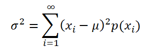
where x i is the value that a random variable can take, and μ is the average value (), p(x) is the probability that the random variable will take the value x.
If a random variable has , then dispersion calculated by the formula:

Dimension variances corresponds to the square of the unit of measurement of the original values. For example, if the values in the sample represent part weight measurements (in kg), then the variance dimension would be kg 2 . This can be difficult to interpret, so to characterize the spread of values, a value equal to square root from variances – standard deviation.
Some properties variances:
Var(X+a)=Var(X), where X is a random variable and a is a constant.
Var(aХ)=a 2 Var(X)
Var(X)=E[(X-E(X)) 2 ]=E=E(X 2)-E(2*X*E(X))+(E(X)) 2 =E(X 2)- 2*E(X)*E(X)+(E(X)) 2 =E(X 2)-(E(X)) 2
This dispersion property is used in article about linear regression.
Var(X+Y)=Var(X) + Var(Y) + 2*Cov(X;Y), where X and Y are random variables, Cov(X;Y) is the covariance of these random variables.
If random variables are independent, then they covariance is equal to 0, and therefore Var(X+Y)=Var(X)+Var(Y). This property of dispersion is used in derivation.
Let us show that for independent quantities Var(X-Y)=Var(X+Y). Indeed, Var(X-Y)= Var(X-Y)= Var(X+(-Y))= Var(X)+Var(-Y)= Var(X)+Var(-Y)= Var( X)+(-1) 2 Var(Y)= Var(X)+Var(Y)= Var(X+Y). This dispersion property is used to construct .
Sample standard deviation
Sample standard deviation is a measure of how widely scattered the values in a sample are relative to their .
A-priory, standard deviation equal to the square root of variances:

Standard deviation does not take into account the magnitude of the values in sample, but only the degree of dispersion of values around them average. To illustrate this, let's give an example.
Let's calculate the standard deviation for 2 samples: (1; 5; 9) and (1001; 1005; 1009). In both cases, s=4. It is obvious that the ratio of the standard deviation to the array values differs significantly between samples. For such cases it is used The coefficient of variation(Coefficient of Variation, CV) - ratio Standard Deviation to the average arithmetic, expressed as a percentage.
In MS EXCEL 2007 and earlier versions for calculation Sample standard deviation the function =STDEVAL() is used, English. name STDEV, i.e. STandard DEViation. From the version of MS EXCEL 2010, it is recommended to use its analogue =STDEV.B() , English. name STDEV.S, i.e. Sample STandard DEViation.
In addition, starting from the version of MS EXCEL 2010, there is a function STANDARDEV.G(), English. name STDEV.P, i.e. Population STandard DEViation, which calculates standard deviation For population. The whole difference comes down to the denominator: instead of n-1 as in STANDARDEV.V(), STANDARDEVAL.G() has just n in the denominator.
Standard deviation can also be calculated directly using the formulas below (see example file)
=ROOT(QUADROTCL(Sample)/(COUNT(Sample)-1))
=ROOT((SUM(Sample)-COUNT(Sample)*AVERAGE(Sample)^2)/(COUNT(Sample)-1))
Other measures of scatter
The SQUADROTCL() function calculates with a sum of squared deviations of values from their average. This function will return the same result as the formula =DISP.G( Sample)*CHECK( Sample) , Where Sample- a reference to a range containing an array of sample values (). Calculations in the QUADROCL() function are made according to the formula:

The SROTCL() function is also a measure of the spread of a data set. The function SROTCL() calculates the average of the absolute values of deviations of values from average. This function will return the same result as the formula =SUMPRODUCT(ABS(Sample-AVERAGE(Sample)))/COUNT(Sample), Where Sample- a link to a range containing an array of sample values.
Calculations in the function SROTCL () are made according to the formula:
