After installing the add-on, you will have a new tab with a function call command. When you click on the command Range Comparison A dialog box appears for entering parameters.
This macro allows you to compare tables of any size and with any number of columns. Table comparisons can be made on one, two, or three columns at a time.
The dialog box is divided into two parts: the left one for the first table and the right one for the second.
To compare tables you need to do the following:
- Specify table ranges.
- Place a checkbox (check mark/bird) under the selected range of tables if the table includes a header (title line).
- Select the columns of the left and right tables for comparison (if the table ranges do not include headings, the columns will be numbered).
- Specify the comparison type.
- Select an option for displaying results.
Table comparison type
 The program allows you to select several types of table comparisons:
Find rows from one table that are missing from another table
When you select this type of comparison, the program looks for rows in one table that are missing in another. If you match tables based on multiple columns, the result will be rows that have a difference in at least one of the columns.
Find matching strings
When you select this type of comparison, the program finds rows that match in the first and second tables. Rows in which the values in the selected comparison columns (1, 2, 3) of one table completely match the values of the columns of the second table are considered to be matching.
An example of how the program works in this mode is shown on the right in the picture.
Match tables based on selection
In this comparison mode, opposite each row of the first table (selected as the main one), the data of the matching row of the second table is copied. If there are no matching rows, the row opposite the main table remains empty.
Comparing tables with four or more columns
If you lack the functionality of the program and need to compare tables by four or more columns, then you can get out of the situation as follows:
- Create an empty column in your tables.
- In new columns using the formula = CONNECT combine the columns you want to compare to.
This way you will end up with 1 column containing the values of multiple columns. Well, you already know how to compare one column.
Say you want to compare versions of a workbook, analyze a workbook for problems or inconsistencies, or see links between workbooks or worksheets. If Microsoft Office 365 or Office Professional Plus 2013 is installed on your computer, the Spreadsheet Inquire add-in is available in Excel.
You can use the commands in the Inquire tab to do all these tasks, and more. The Inquire tab on the Excel ribbon has buttons for the commands described below.
If you don't see the Inquire tab in the Excel ribbon, see Turn on the Spreadsheet Inquire add-in .
Compare two workbooks
The Compare Files command lets you see the differences, cell by cell, between two workbooks. You need to have two workbooks open in Excel to run this command.
Results are color coded by the kind of content, such as entered values, formulas, named ranges, and formats. There"s even a window that can show VBA code changes line by line. Differences between cells are shown in an easy to read grid layout, like this:

The Compare Files command uses Microsoft Spreadsheet Compare to compare the two files. In Windows 8, you can start Spreadsheet Compare outside of Excel by clicking Spreadsheet Compare on the Apps screen. In Windows 7, click the Windows Start button and then > All Programs > Microsoft Office 2013 > Office 2013 Tools > Spreadsheet Compare 2013.
To learn more about Spreadsheet Compare and comparing files, read Compare two versions of a workbook.
Analyze a workbook
The Workbook Analysis command creates an interactive report showing detailed information about the workbook and its structure, formulas, cells, ranges, and warnings. The picture here shows a very simple workbook containing two formulas and data connections to an Access database and a text file.

Show workbook links
Workbooks connected to other workbooks through cell references can get confusing. Use the to create an interactive, graphical map of workbook dependencies created by connections (links) between files. The types of links in the diagram can include other workbooks, Access databases, text files, HTML pages, SQL Server databases, and other data sources. In the relationship diagram, you can select elements and find more information about them, and drag connection lines to change the shape of the diagram.
This diagram shows the current workbook on the left and the connections between it and other workbooks and data sources. It also shows additional levels of workbook connections, giving you a picture of the data origins for the workbook.

Show worksheet links
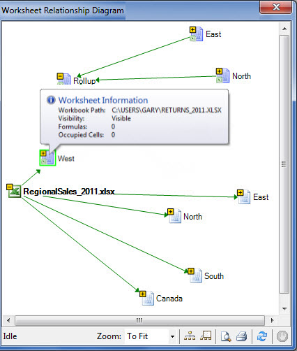
Got lots of worksheets that depend on each other? Use the to create an interactive, graphical map of connections (links) between worksheets both in the same workbook and in other workbooks. This helps give you a clearer picture of how's your data might depend on cells in other places.
This diagram shows the relationships between worksheets in four different workbooks, with dependencies between worksheets in the same workbook as well as links between worksheets in different workbooks. When you position your pointer over a node in the diagram, such as the worksheet named "West" in the diagram, a balloon containing information appears.
Show cell relationships
To get a detailed, interactive diagram of all links from a selected cell to cells in other worksheets or even other workbooks, use the Cell Relationship tool. These relationships with other cells can exist in formulas, or references to named ranges. The diagram can cross worksheets and workbooks.
This diagram shows two levels of cell relationships for cell A10 on Sheet5 in Book1.xlsx. This cell is dependent on cell C6 on Sheet 1 in another workbook, Book2.xlsx. This cell is a precedent for several cells on other worksheets in the same file.

To learn more about viewing cell relationships, read See links between cells.
Clean excess cell formatting
Ever open a workbook and find it loads slowly, or has become huge? It might have formatting applied to rows or columns you aren't aware of. Use the Clean Excess Cell Formatting command to remove excess formatting and greatly reduce file size. This helps you avoid "spreadsheet bloat," which improves Excel"s speed.
Manage passwords
If you"re using the Inquire features to analyze or compare workbooks that are password protected, you"ll need to add the workbook password to your password list so that Inquire can open the saved copy of your workbook. Use the Workbook Passwords command on the Inquire tab to add passwords, which will be saved on your computer. These passwords are encrypted and only accessible by you.
Sometimes there is a need to compare two MS Excel files. This could be finding price discrepancies for certain positions or a change in any indications is not important, the main thing is that it is necessary to find certain discrepancies.
It would not be amiss to mention that if there are a couple of records in the MS Excel file, then there is no point in resorting to automation. If the file contains several hundred, or even thousands of records, then it is impossible to do without the help of the computing power of a computer.
Let's simulate a situation where two files have the same number of lines, and the discrepancy must be looked for in a specific column or in several columns. This situation is possible, for example, if you need to compare the price of goods according to two price lists, or compare measurements of athletes before and after the training season, although for such automation there must be a lot of them.
As a working example, let's take a file with the performance of fictitious participants: 100-meter run, 3000-meter run, and pull-ups. The first file is a measurement at the beginning of the season, and the second is the end of the season.
The first way to solve the problem. The solution is only using MS Excel formulas.
Since the records are arranged vertically (the most logical arrangement), it is necessary to use the function. If you use horizontal placement of records, you will have to use the function.
To compare 100 meter running performance, the formula is as follows:
=IF(VLOOKUP($B2,Sheet2!$B$2:$F$13,3,TRUE)<>D2;D2-VLOOKUP($B2;Sheet2!$B$2:$F$13,3,TRUE);"No difference")
If there is no difference, a message is displayed that there is no difference; if there is a difference, then the value at the end of the season is subtracted from the value at the beginning of the season.
The formula for the 3000 meter run is as follows:
=IF(VLOOKUP($B2,Sheet2!$B$2:$F$13,4,TRUE)<>E2;"There is a difference";"There is no difference")
If the final and initial values are not equal, a corresponding message is displayed. The formula for pull-ups can be similar to any of the previous ones; there is no point in giving it additionally. The final file with the discrepancies found is shown below.
A little clarification. To make the formulas easier to read, data from two files was moved into one (on different sheets), but this could not have been done.
Video comparing two MS Excel files using and functions.
The second way to solve the problem. Solution using MS Access.
This problem can be solved if you first import MS Excel files into Access. As for the method of importing external data itself, there is no difference in finding different fields (any of the presented options will do).
The latter is a connection between Excel and Access files, so when you change data in Excel files, discrepancies will be found automatically when you run a query in MS Access.
The next step after importing is to create relationships between tables. As a connecting field, select the unique field “Item No.”
The third step is to create a simple select query using the Query Builder.
In the first column we indicate which records need to be displayed, and in the second - under what conditions the records will be displayed. Naturally, for the second and third fields the actions will be similar.
Video comparing MS files to Excel using MS Access.
As a result of the manipulations performed, all records are displayed, with different data in the field: “Running 100 meters.” The MS Access file is presented below (unfortunately, SkyDrive does not allow embedding as an Excel file)
These two methods exist for finding discrepancies in MS Excel tables. Each has both advantages and disadvantages. Obviously, this is not an exhaustive list of comparisons between the two Excel files. We are waiting for your suggestions in the comments.
Question from a user
Hello!
I have one task, and for the third day now I’ve been racking my brains - I don’t know how to complete it. There are 2 tables (about 500-600 rows in each), you need to take the column with the name of the product from one table and compare it with the name of the product from the other, and if the products match, copy and paste the value from table 2 into table 1. Confusedly explained , but I think you’ll understand the task from the photo ( approx. : the photo was cut out by censorship, it’s still personal information).
Thank you in advance. Andrey, Moscow.
Good day everyone!
What you described refers to fairly popular tasks that are relatively easy and quick to solve using Excel. All you need to do is put your two tables into the program and use the VLOOKUP function. More about her work below...
An example of working with the VLOOKUP function
As an example, I took two small signs, they are shown in the screenshot below. In the first table (columns A, B- product and price) no data on the column B; in the second, both columns (product and price) are filled in. Now you need to check the first columns in both tables and automatically, if a match is found, copy the price to the first table. It seems like a simple task...

How to do it...
Place the mouse pointer in the cell B2- that is, in the first cell of the column where we have no value and write the formula:
=VLOOKUP(A2,$E$1:$F$7,2,FALSE)
A2- the value from the first column of the first table (what we will look for in the first column of the second table);
$E$1:$F$7- a completely selected second table (in which we want to find and copy something). Pay attention to the "$" sign - it is necessary so that when copying the formula, the cells of the selected second table do not change;
2 - the number of the column from which we are copying the value (note that our selected second table has only 2 columns. If it had 3 columns, then the value could be copied from the 2nd or 3rd column);
LIE- we are looking for an exact match (otherwise the first similar one will be substituted, which obviously does not suit us).

Actually, you can adjust the finished formula to your needs by slightly changing it. The result of the formula is presented in the picture below: the price was found in the second table and entered in auto mode. Everything is working!

To set the price for other product names, simply extend (copy) the formula to other cells. Example below.

After which, as you can see, the first columns of the tables will be compared: from the rows where the cell values coincide, the necessary data will be copied and substituted. In general, it is clear that tables can be much larger!

Note: I must say that the VLOOKUP function is quite demanding on computer resources. In some cases, with an excessively large document, it may take quite a long time to compare tables. In these cases, it is worth considering either other formulas or completely different solutions (each case is individual).
That's all, good luck!